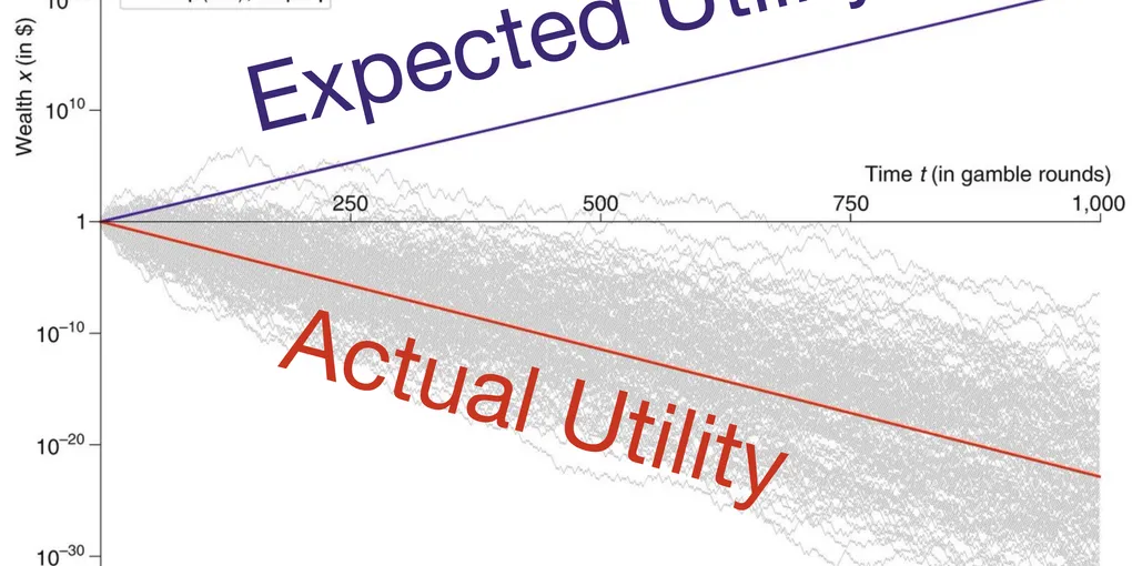
Expected-utility maximizers don't maximize utility.


Ergodicity economics is an umbrella term for addressing issues in economics research by carefully considering the ergodicity problem — that’s the problem that the expected value of something may be different from its time average. One key finding which illustrates the field’s significance within the history of economics is the mapping between utility functions and ergodicity transformations. This mapping provides a physical (as opposed to psychological) interpretation of where utility functions really come from. It also highlights a weakness of expected-utility theory: agents who follow the prescriptions of expected-utility theory do not maximize utility in the long run; agents who follow the prescriptions of ergodicity economics, on the other hand, do maximize utility in the long run.
Perhaps the simplest way to explain the problem is to consider the infamous coin toss. Here, expected wealth goes up as time passes, while wealth itself is guaranteed to go down in the long run. In terms of expected-utility theory this is problematic. Imagine a linear-utility agent, meaning a so-called risk-neutral agent, who just cares about dollars, not some non-linear function of dollars. Because wealth is then the same as utility, expected utility goes up in the infamous coin toss, but utility itself is guaranteed to go down. We conclude: expected utility is a bad thing to maximize if you want to maximize utility.
This is worth saying again: if you want utility, don’t optimize expected utility because you’re bound to lose actual utility. How is this possible? Well, broken ergodicity. Expected utility is an average over the statistical ensemble, and that looks rosy. But you don’t have access to the average over the statistical ensemble, only to one realization. And in each individual realization you’re guaranteed to lose as time goes on. If this is puzzling, then ergodicity economics is for you. It’s all about understanding this deep puzzle and using our understanding of it to make sense of the real world via modern mathematical models.
Mini history of decision theory
Expected-value theory
Historically, the first fully quantitative model (1650s) of human behavior under risk was expected-value theory (EVT). It was invented in the context of simple gambling tasks, like tossing a coin to win or lose some amount of money. Let’s say someone offers me such a gamble, and I want to apply the EVT framework. I would follow these steps:
-
model the gamble on offer as a random variable whose possible values are the possible net changes in dollar wealth (like net-win $5 or net-lose $3) with sensible probabilities (like 50/50 for a fair coin toss).
-
Compute the expected value of the random variable.
-
If this is positive, accept the gamble; otherwise reject.
Expected-utility theory
It was soon noticed that this model was not a good description of what real people do. Often, we reject gambles with positive expected value. This realization led to the development of expected-utility theory (EUT, 1730s). In this framework, it is posited that people don’t value money linearly. To reflect this, a “utility function” is defined. It increases with wealth, , and is usually non-linear to account for the failure of expected-value theory. For instance, if the utility function is concave as is typically assumed, then a given dollar loss decreases utility more than a dollar gain of the same size increases utility. Two-hundred-fifty years later concavity was repackaged as the alliterative phrase “losses loom larger than gains.”
The steps of expected-utility theory are very similar to those of expected-value theory.
-
Model the changes in utility as a random variable (given by the transformation ).
-
Compute its expected value.
-
Accept the gamble if the expected utility change is positive.
The message from expected-utility theory is this: you don’t really care about dollars, you care about the usefulness of dollars.
The promise of expected-utility theory is, of course: specify your utility function, stick it into the formalism, follow what the formalism tells you to do, and you will maximize utility (though possibly not wealth).
But EUT does not keep its promise. You can see this immediately: utility is an increasing function of wealth. It’s non-linear, but we still prefer more wealth to less wealth. Therefore, more wealth always means more utility. If the expected-utility framework does not maximize wealth, then it also doesn’t maximize utility.
So what is going on? In a second, we will go through an explicit example calculation, but before we do that, here is the problem: expected-utility theory maximizes expected utility. But expected anything is something very strange — physically (if that’s the right word), it’s an average over parallel universes. Perhaps it’s better to say that it has no immediate physical real-world meaning. Consequently, maximizing it doesn’t guarantee anything about the real world; only about a mathematical ensemble of hypothetically possible worlds. Sometimes such an imagined ensemble has real-world significance, but if that is the case, it has to be carefully established, not simply assumed.
The leverage problem
Since this is all a bit abstract, let’s move on to a concrete computation. The example is a standard problem every ergodicity economist, or indeed finance student, sees somewhere early on in his or her education — leveraged geometric Brownian motion.
Here, an agent gets to decide how much risk to take by choosing its exposure to a risky asset whose value, follows geometric Brownian motion,
(Eq. 1)
with the usual nomenclature and notation: is called the drift, volatility, time, and is a Wiener process.
The agent chooses how much of its wealth to invest in this asset — that’s the so-called leverage problem. In other words, the agent chooses the leverage, , in the wealth process
(Eq. 2)
For simplicity, we have assumed here that the risk free interest rate is zero — the agent can borrow for free and receives nothing for deposits. As a consequence, if the agent chooses to invest nothing in the risky asset, leverage , it will gain nothing, and wealth is constant, . With leverage , everything is invested in the risky asset and Eq.2 looks just like Eq.1, and with leverage both the drift and the volatility of the agent’s wealth are twice as large as those of the risky asset, and so on.
Ergodicity economics solution
Ergodicity economics tells us how to solve the leverage problem [1] by choosing the leverage which guarantees greatest wealth in the long run. After a little Ito calculus we arrive at the time-optimal leverage, which is
(Eq. 3) .
At this leverage, our wealth grows faster than at any other leverage as time passes.
Expected-utility theory solution
Expected-utility theory is conceptually different: it finds the leverage which maximizes expected utility, not the leverage that makes wealth grow fastest. Because utility is monotonic in wealth, agents who follow the recommendations of ergodicity economics are guaranteed to obtain more utility in the long run than expected-utility agents.
That’s a bit crazy — expected-utility theory prides itself on helping people obtain utility, and ergodicity-economics is often criticized for focusing on wealth and not utility. Nonetheless, ergodicity economics guarantees not only greater wealth but also greater utility in the long run.
We illustrate this by computing the optimal leverage according to EUT (which maximizes expected utility) for a popular class of utility functions, called isoelastic utilities, which have the following form
(Eq. 4) ,
where is usually called the risk-aversion parameter — the greater it is, the more an EUT agent will shy away from risk. We now compute the expected change in this utility function, given the wealth dynamic, Eq.2, and then find the leverage for which it is maximized. Using the utility function in Eq.4, we apply Ito’s formula to find the changes in utility,
(Eq. 5)
.
Next, we drop the higher-order terms (h.o.t) and substitute the first and second derivatives of the utility function. They are and .
Substituting in Eq.5, we find that the changes in utility are
(Eq. 6)
The expected value of the utility change is now trivially calculated (it just amounts to dropping the term with ) as
(Eq. 7) .
It only remains to maximize with respect to the leverage,
(Eq. 8) ,
which is zero at
(Eq. 9) ,
implying the EUT-optimal leverage
(Eq. 10) .
The value of this EUT-optimal leverage is entirely set by the utility function of the agent, here represented by its risk-aversion parameter . Depending on the agent’s psychology and intrinsic preferences, EUT-optimal leverage can take any value from negative to positive infinity. Therefore, except for the small range of values , an agent behaving according to EUT will destroy its wealth because it will choose a leverage at which wealth is systematically gambled away exponentially fast. This is an embarrassing feature of EUT. It destroys wealth and therefore the utility it aims to maximise.
Two concepts of optimal
We now have two optimal solutions: the EE solution guarantees maximum actual wealth and maximum actual utility in the long run; the EUT solution guarantees maximum expected utility but this is unrelated to actual wealth and actual utility.
To let you explore what these equations mean, we’ve written App 1 below, where you can choose a utility function by setting the risk-aversion parameter and the time scale over which you want to simulate. Hit “Plot utility function” to see what looks like. Next, hit “Simulate agents:” the wealths and utilities of two agents will be displayed, as the agents leverage according to their optimality criteria (the risky asset follows Eq.1 with and ). One agent chooses its leverage according to EE (blue lines) and the other according to EUT (orange lines). Of course, in a simulation, which is always finite, there is a chance that the EUT agent ends up with more utility than the EE agent. In the long-time limit this is impossible unless the EUT agent uses as the utility function something we call the ergodicity transformation (which is determined by the dynamic, not by intrinsic preferences). In that special case, EUT agents are guaranteed to behave exactly as EE agents. So we arrive at the curious situation where either EUT leads to less utility than EE; or else EUT is restricted to be equivalent to EE in which case the EUT agents obtain the same utility as the EE agents.
App 1: Set the risk aversion parameter and the time over which you want to simulate.
This raises the question what EUT has to offer beyond EE. EUT is by its nature a curve-fitting exercise: there’s nothing to predict the utility function, and nothing to explain why people have the utility function they have. It has also been found to do very poorly predictively, with a major study, reviewing seven decades of empirical work, concluding that its “power to predict out-of-sample is in the poor to non-existent range.”[2]
As we have shown here, EUT is unable to do what it set out to do: maximise utility. With this in mind, the empirical failure of EUT may be less surprising.
EE is different. The ergodicity transformation is determined by the dynamics, it’s not a free parameter, and at this level there is no fitting involved. EE has been found to do well in predicting behavior.
Perhaps EE clarifies why EUT fails, predictively speaking: EUT does not take the dynamics into account but they are an important reason for people to behave the way they do. Inferring the utility function from observed behavior (called “revealed preferences” in economics) is not terribly meaningful in a predictive sense because the dynamic circumstances of an observed individual may change from the time its utility function was fitted to the time that utility function is used to make predictions.
The beauty of EE is that we know precisely why it does what, what it explains, and what predictions we can expect from it. The perspective offered by EE leaves us with a stark choice when it comes to EUT. Either EUT fails to maximise utility over time, challenging its raison d’etre; or EUT becomes precisely ergodicity economics, in which case it adds nothing.
Curious about Ergodicity Economics? We recommend the textbook An Introduction to Ergodicity Economics.
You may also want to join our mailing list for all things ergodicity economics.
References:
[1] see Chapter 10, An Introduction to Ergodicity Economics (2025), O. Peters and A. Adamou.
[2] see p.3, Risky Curves - On the empirical failure of expected utility (2014), D. Friedman, R. M. Isaac, D. James, S. Sunder.

Discuss this post on the EE Discord server.
Last updated on